Pub figures
Some of figures from different segments of the analysis were colated for the manuscript.
Here we present the code/process used to put them together.
Treatments analysis
Number of treatments and proportion of the total dose used in fungicide trials.
Load packages
list.of.packages <-
  c(
    "tidyverse",
    "readxl",
    "devtools",
    "ggpubr",
    "zoo",
    "kableExtra",
    "conflicted",
    "here",
    "lubridate",
    "magick",
    "egg",
    "conflicted",
    "poppr",
    "magick"
  )

new.packages <-
  list.of.packages[!(list.of.packages %in% installed.packages()[, "Package"])]

#Download packages that are not already present in the library
if (length(new.packages))
  install.packages(new.packages)

packages_load <-
  lapply(list.of.packages, require, character.only = TRUE)

#Print warning if there is a problem with installing/loading some of packages
if (any(as.numeric(packages_load) == 0)) {
  warning(paste("Package/s: ", paste(list.of.packages[packages_load != TRUE], sep = ", "), "not loaded!"))
} else {
  print("All packages were successfully loaded.")
}
## [1] "All packages were successfully loaded."rm(list.of.packages, new.packages, packages_load)
conflict_prefer("filter", "dplyr")
#if instal is not working try
#install.packages("ROCR", repos = c(CRAN="https://cran.r-project.org/"))Weather
df <-
  read_csv(
    here::here("data", "weather" , "hly375.csv"),
    col_types = cols(
      clamt = col_skip(),
      clht = col_skip(),
      vis = col_skip(),
      w = col_skip(),
      ww = col_skip()
    ),
    skip = 17
  )

df$date <-
  lubridate::dmy_hm(df$date)
df<- add_column(df, short_date = as.Date(df$date), .after=1)
df<- add_column(df, year = year(df$date), .after=2)
df<- add_column(df, month = month(df$date), .after=3)
df<- add_column(df, day = day(df$date), .after=4)


infil_gap <- 8 #Maximum length of the infill gap
df$temp <-
  round(na.spline(df$temp, na.rm = FALSE, maxgap = infil_gap), 1)
df$rhum <-
  round(na.spline(df$rhum, na.rm = FALSE, maxgap = infil_gap), 0)
df$rhum  <- sapply(df$rhum, function(x)
  ifelse(x > 100, x <- 100, x))

df <-
  df %>%
  filter(year %in% 2016:2019)%>%
  filter(month %in% c(4:9))

#Check if the imputation worked
df %>%
  summarize(
    NA_rain = sum(is.na(rain)),
    NA_temp = sum(is.na(temp)),
    NA_rhum = sum(is.na(rhum))
  )%>%
  kable(format = "html") %>%
kableExtra::kable_styling(latex_options = "striped",full_width = FALSE)| NA_rain | NA_temp | NA_rhum |
|---|---|---|
| 2 | 0 | 0 |
#Only two missing values for rain should not be a problem, so we will just do a linear interpolation
df$rain <-
  round(na.approx(df$rain, na.rm = FALSE, maxgap = infil_gap), 1)


dfday <-
  df %>%
  group_by(year, month, short_date) %>%
  summarize(
    mintemp = round(min(temp), 1),
    minrhum = round(min(rhum), 1),
    temp = round(mean(temp), 1),
    rain = sum(rain),
    rhum = round(mean(rhum), 1),
    meantemp = round(mean(temp), 1),
    meanrhum = round(mean(rhum), 1)
  )

#REad disease data
disdata <-
read_rds( path = here::here("results", "dis", "Duration of the epidemics in years.Rdata"))
colnames(disdata) <-
  c("year", "disout", "disend")
dfday <-
  left_join(dfday, disdata, by = "year")

# rolling mean
rlmean <- 10
dfday$wrhum <- zoo::rollmean(dfday$meanrhum, rlmean, mean, align = 'center', fill = NA)
dfday$wtemp <- zoo::rollmean(dfday$mintemp, rlmean, mean, align = 'center', fill = NA)

#conducive days
templine <- 10
dfday <-
  dfday %>%
  mutate(condday = ifelse( wtemp>=templine&rain>=.2&rhum>=80& short_date<disout, 50,NA))

#sum of conditions prior to outbreak
dfday <-
dfday %>%
  group_by(year) %>%
  summarise(consum= sum(condday/50, na.rm = TRUE )) %>%
  left_join(dfday,., by = "year")

#LAbels for cumulative sum of critical days
dfday <-
dfday %>%
  mutate(symptoms = paste0("Symptoms (", consum, " cond. days)"))


linesize <- .35 #size of the line for variables

dfday %>%
  mutate(rain = ifelse(rain == 0, NA, rain)) %>%
  rename(date = short_date) %>%
  ggplot() +
  geom_point(aes(disout, 46),shape =2, size = 1.5, fill ="black")+
  geom_point(aes(disend, 46),shape =2, size = 1.5, fill ="black")+
  geom_point(aes(date, condday), shape = 3,size = .55)+
  geom_line(
    aes(
      x = date,
      y = rhum,
      colour = "Relative humidity (%)"
    ),
    size = linesize
  ) +
  geom_line(aes(
    x = date,
    y = temp,
    colour = "Temperature (˚C)",
  ),
  size = linesize) +
  geom_line(aes(
    x = date,
    y = wtemp,
    colour = "Rolling mean temp. (˚C)"
  ),
  linetype = "dashed",
  size = linesize) +
  geom_col(
    aes(date,
        rain,
        fill = "Total precipitation (mm/day)"),
    size = 1.2 ,
    inherit.aes = TRUE,
    width = 0.8
  ) +
  scale_colour_manual(
    "Daily weather:",
    values = c(
      "Relative humidity (%)" = "#0EBFE9",
      "Temperature (˚C)" = "#ED2939",
      "Rolling mean temp. (˚C)"= "darkred"
    )
  ) +
  scale_fill_manual(name= NA, values = c("Total precipitation (mm/day)" = "blue")
  ) +
  scale_y_continuous( breaks = seq(0,100,10), limits = c(-1,100),expand = c(0, 0))+
  scale_x_date(date_labels = "%b", date_breaks = "1 month",expand = c(.03, .04))+
  facet_wrap( ~ year, scales = "free", ncol = 1,strip.position="right") +
  guides(fill=guide_legend(nrow=1,byrow=TRUE,title.position = "top"),
         color=guide_legend(nrow=1,byrow=TRUE,title.position = "top"),
         linetype=guide_legend(nrow=1,byrow=TRUE,title.position = "top"))+
  theme_bw()+
  theme(
    text = element_text(size=10.8),
    # axis.text.x = element_blank(),
    # axis.ticks.x = element_blank(),
    axis.title.y = element_blank(),
    axis.title.x = element_blank(),
    # axis.text.y = element_blank(),
    # axis.ticks.y = element_blank(),
    legend.position = "top",
    strip.background =element_rect(colour = "black",size=0.75),
    strip.placement = "outside",
    legend.title = element_blank(),
    panel.grid.minor =   element_blank(),
    panel.grid.major =   element_line(colour = "lightgray",size=linesize),
    plot.margin = margin(0, 0, 0, 0, "cm"),
    panel.spacing.y=unit(0, "lines"),
    legend.box.spacing = unit(0.1, 'cm'),
    legend.margin = margin(0, 0, 0, 0, "cm"),
  )+
  geom_text(aes(label= symptoms, y = 39, x = disout),size = 2.5)+
  geom_text(aes(label= "Last assesment", y = 39, x = disend-1.5),size = 2.5)+
  ggsave(filename= here::here("results", "wth", "all_wth_dis.png"),
         width = 6.5, height =8, dpi = 720)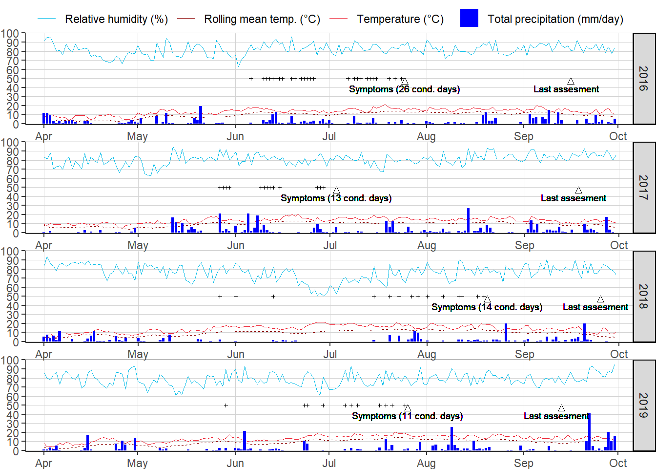
Population frequencies and DAPC analysis
GGplots from the frequency analysis wee colated using ‘ggpubr’ and DAPC plots using ‘magick’.
plotls <- readRDS(file = here::here("results", "gen", "freq","freq_plots.RDS"))

plotls <-
  lapply(plotls, function(x)
    x <- x+
      theme(plot.background = element_rect(size=.3,linetype="solid",color="black")))

plotf <-
ggpubr::ggarrange(plotlist = plotls,
                  heights = c(1,1,1),
                  # labels = c("r","rr"),
                  nrow = 3)

ggsave(
  plot = plotf,
  filename = here::here("results", "gen", "freq", "Freq_all.png"),
  width = 2.9,
  height = 9,
  dpi = 820
)


# Read external images
#shell.exec(here::here("results", "gen","dapc", "treatment.png"))
t = image_read(here::here("results", "gen","dapc", "treatment.png"))
v = image_read(here::here("results", "gen","dapc", "variety.png"))
y = image_read(here::here("results", "gen","dapc", "year.png"))
imgs = c(v,t,y)

# concatenate them left-to-right (use 'stack=T' to do it top-to-bottom)
side_by_side = image_append(imgs, stack=T)

# save
image_write(side_by_side,
            path = here::here("results", "gen","dapc","dapcs",  "full_dapc.png"),
            format = "png")


#add the frequency plots
f = image_read(here::here("results", "gen", "freq", "Freq_all.png"))
dapcs = image_read(here::here("results", "gen","dapc","dapcs", "full_dapc.png"))

#Append and save the image

scale <- paste0("x", 7380)
# concatenate them left-to-right (use 'stack=T' to do it top-to-bottom)
side_by_side <-  image_append(c(f, image_scale(dapcs, scale)), stack = FALSE)


image_write(side_by_side,
            path = here::here("results", "gen","dapc","dapcs",  paste0(scale, "full.png")),
            format = "png",
            # width = 4500,
            # height = 3700
)

#To open the figure in external viewer uncoment the following lines
#shell.exec(here::here("results", "gen","dapc","dapcs", paste0(scale, "full.png")))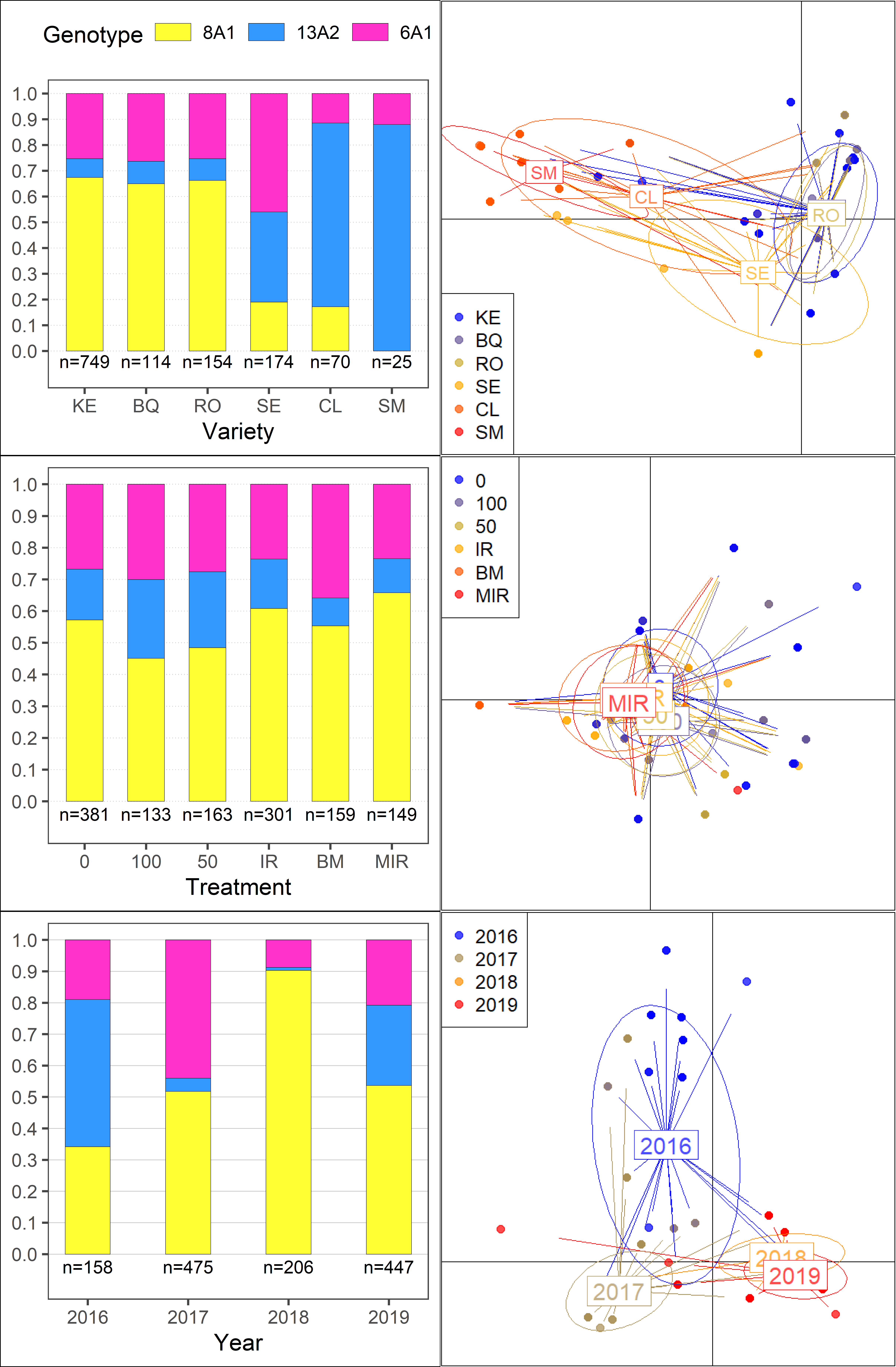
Final figure
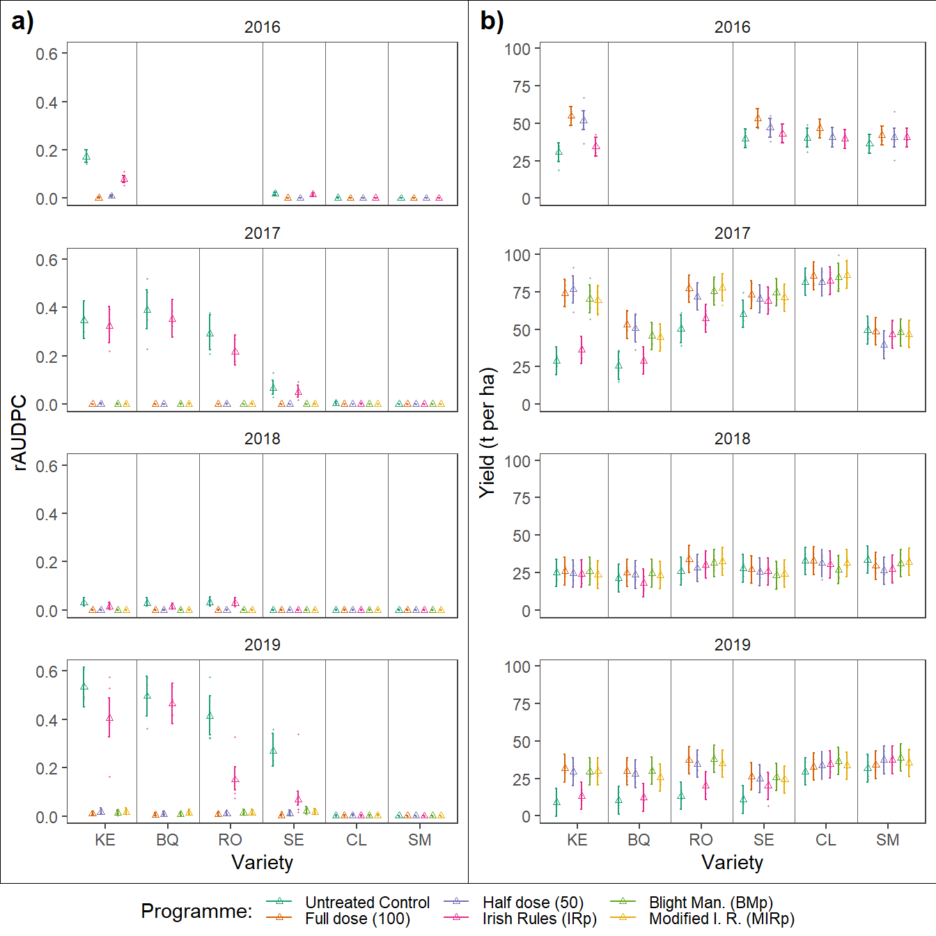
Disease and yield
Results of the foliar disease controll yield analysis were colated in single figure using ‘magick’ package.
dd <-
  readRDS( file = here::here("results", "dis",  "dis_fin.RDS"))
yd <-
  readRDS( file = here::here("results", "yield",  "yld_fin.RDS"))
yld <-
  readRDS( file = here::here("results", "yield",  "yld_dat_fin.RDS"))
audpc_data <-
  readRDS( file = here::here("results", "dis",  "dis_audpc_fin.RDS"))

dodging <-  .8

pdfin <-
dd %>%
  mutate(
    line_positions = as.numeric(factor(variety, levels = unique(variety))),
    line_positions = line_positions + .5,
    line_positions = ifelse(line_positions == max(line_positions), NA, line_positions),
    line_positions = ifelse(year == 2016 &
                              variety == "SM", 5.5, line_positions),
    line_positions = ifelse(year == 2016 &
                              variety == "CL", 4.5, line_positions),
    line_positions = ifelse(year == 2016 &
                              variety == "SE", 3.5, line_positions),
    line_positions = ifelse(year == 2016 &
                              variety == "KE", 1.5, line_positions)

  ) %>%
  ggplot(data = ., aes(x = variety, y = prop)) +
  geom_errorbar(
    aes(
      ymin = lower.CL,
      ymax = upper.CL,
      group = treatment,
      color = treatment
    ),
    position = position_dodge(width = dodging),
    width = .2
  ) +
  geom_point(
    aes(y = prop, group = treatment, color = treatment),
    size = 1,
    shape = 2,
    position = position_dodge(width = dodging)
  )+
  geom_point(
    data = subset(audpc_data),
    aes(y = rAUDPC_adj, color = treatment, group = treatment),
    size = .2,
    alpha = .5,
    position = position_dodge(width = dodging)
  ) +
  facet_wrap(~ year, ncol = 1)+
  scale_color_brewer("Programme:", palette = "Dark2") +
  theme_article() +
  theme(legend.position = "bottom",
        text = element_text(size = 13)) +
    geom_vline(aes(xintercept = line_positions),
             size  = .2,
             alpha = .6) +
  labs(colour = "Programme:",
       x = "Variety",
       y = "rAUDPC")


  ggsave(plot = pdfin,
    filename = here::here("results", "dis", "Effects final ver.png"),
    width = 4,
    height = 7,
    dpi = 620
  )


 py_fin <-
  yd %>%
  mutate(
    line_positions = as.numeric(factor(variety, levels = unique(variety))),
    line_positions = line_positions + .5,
    line_positions = ifelse(line_positions == max(line_positions), NA, line_positions),
    line_positions = ifelse(year == 2016 &
                              variety == "SM", 5.5, line_positions),
    line_positions = ifelse(year == 2016 &
                              variety == "SE", 4.5, line_positions)
  ) %>%
  ggplot(data = ., aes(x = variety, y = lsmean)) +
  geom_errorbar(
    aes(
      ymin = lower.CL,
      ymax = upper.CL,
      group = treatment,
      color = treatment
    ),
    position = position_dodge(width = dodging),
    width = .2
  ) +
  geom_point(
    aes(y = lsmean, group = treatment, color = treatment),
    size = 1,
    shape = 2,
    position = position_dodge(width = dodging)
  ) +
  geom_point(
    data = yld,
    aes(y = marketable, color = treatment, group = treatment),
    size = .2,
    alpha = .5,
    position = position_dodge(width = dodging)
  ) +
  facet_wrap(~ year, ncol = 1) +
  scale_color_brewer("Programme:", palette = "Dark2") +
  theme_article() +
  theme(legend.position = "bottom",
        text = element_text(size = 13)) +
  geom_vline(aes(xintercept = line_positions),
             size  = .2,
             alpha = .6) +
  labs(colour = "Programme:",
       x = "Variety",
       y = "Yield (t per ha)")

py_fin <-
py_fin+
  facet_wrap(~ year, ncol = 1)


ggsave(
  py_fin,
  filename = here::here("results", "yield", "Effects final ver.png"),
  width = 3.5,
  height = 7,
  dpi = 620
)


plotls <- list(pdfin,py_fin)
plotls <-
  lapply(plotls, function(x)
    x <- x+
      theme(plot.background = element_rect(size=.3,linetype="solid",color="black"),
            text = element_text(size= 11))
  )

ggpubr::ggarrange(plotlist = plotls,
                  widths = c(2.5,2.5),
                  heights = c(.5,.5),
                  labels = c("a)","b)"),
                  nrow = 1,
                  common.legend = TRUE,
                  legend = "bottom")+
  ggsave(filename= here::here("results", "dis", "dis_yld.png"),
         width = 7.5, height =10, dpi = 620)