Population Data
Popoulation analysis
Presentation of the sampling and a descriptive analysis of the samples collected.
Load packages
list.of.packages <-
  c(
    "tidyverse",
    "devtools",
    "egg",
    "tableHTML",
    "kableExtra",
    "conflicted"
  )

new.packages <-
  list.of.packages[!(list.of.packages %in% installed.packages()[, "Package"])]

#Download packages that are not already present in the library
if (length(new.packages))
  install.packages(new.packages)

packages_load <-
  lapply(list.of.packages, require, character.only = TRUE)

#Print warning if there is a problem with installing/loading some of packages
if (any(as.numeric(packages_load) == 0)) {
  warning(paste("Package/s: ", paste(list.of.packages[packages_load != TRUE], sep = ", "), "not loaded!"))
} else {
  print("All packages were successfully loaded.")
}
## [1] "All packages were successfully loaded."rm(list.of.packages, new.packages, packages_load)
#Resolve conflicts
if(c("MASS", "dplyr")%in% installed.packages())conflict_prefer("select", "dplyr")
if(c("stats", "dplyr")%in% installed.packages()){
conflict_prefer("filter", "dplyr")
conflict_prefer("select", "dplyr")
}
#if instal is not working try
#install.packages("package_name", repos = c(CRAN="https://cran.r-project.org/"))Data import
Import the data and set the levels of the treatment (3 fixed and 3 variable doses) and variety (susceptible to resistant).
A single isolate belonging to 36A2 was excluded from further analysis due to low sample size.
samples <-
  readRDS(file = here::here("data", "gen data", "final", "gendata.rds") )

samples <-
samples %>%
  filter(Genotype != "36A2")

samples <-
samples %>%
  mutate(Genotype = factor(Genotype, levels = c( "8A1","13A2","6A1" )))

samples$date <- as.Date(samples$date, "%m/%d/%Y")

paste( "The data set is consisted of", nrow(samples), "genotyped samples")
## [1] "The data set is consisted of 1286 genotyped samples"#Prepare the poulation strata initials
samples$treatment <-
factor(samples$treatment, levels = c("0", "100","50","IR","BM" ,"MIR"))
samples <-
samples %>%
mutate(variety = factor(variety, levels =c("KE","BQ", "RO", "SE", "CL","SM"))) Sampling dates and number of samples.
samp_dates <-
samples %>%
  group_by(year, date) %>%
  summarise(`No. of Samples` = n()) %>%
  rename(Year = year, Date = date)

write_csv(samp_dates, here::here("results", "gen", "Sampling dates&counts.csv"))

samp_dates %>%
kableExtra::kable()| Year | Date | No. of Samples |
|---|---|---|
| 2016 | 2016-09-24 | 158 |
| 2017 | 2017-07-03 | 12 |
| 2017 | 2017-07-14 | 5 |
| 2017 | 2017-07-20 | 3 |
| 2017 | 2017-07-31 | 38 |
| 2017 | 2017-08-10 | 154 |
| 2017 | 2017-08-23 | 138 |
| 2017 | 2017-09-13 | 125 |
| 2018 | 2018-08-20 | 3 |
| 2018 | 2018-08-28 | 7 |
| 2018 | 2018-09-05 | 31 |
| 2018 | 2018-09-24 | 165 |
| 2019 | 2019-08-14 | 250 |
| 2019 | 2019-08-27 | 197 |
s_tab <-
 samples %>%
   group_by(year,variety, treatment) %>%
   summarise(count = n()) %>%
   spread(variety, count) %>%
  rename(Year = year,
         Prog. = treatment) %>%
  replace(is.na(.), 0) %>%
  ungroup()

write_csv(s_tab, here::here("results", "gen", "Summary of isolates.csv"))
# s_tab %>%
# kable(format = "html") %>%
# kableExtra::kable_styling(latex_options = "striped")

years <-
s_tab %>%
group_by(Year) %>%
  summarise(counts =n()) %>%
  dplyr::select(counts) %>%
  unlist
year_names <-  unique(s_tab$Year)

tab <-
dplyr::select(s_tab, -c(Year)) %>%
tableHTML::tableHTML(.,
                     rownames = FALSE,
                     row_groups = list(c(years), c(year_names)),
                     # widths = c(50, 60, 70, rep(40, 6))
                     ) %>%
   # add_css_header(css = list('background-color', 'lightgray'), headers = c(1:ncol(s_tab)+1)) %>%
  add_css_row(css = list('background-color', 'lightgray'),
              rows = c(which(s_tab$Year %in% c(2017, 2019))+1)) %>%
  add_theme('scientific')%>%
  tableHTML_to_image(.,file =here::here("results", "gen", "Summary of isolates.png"),
                     type = "png")

rm(years, s_tab)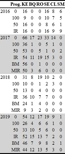
Table1
Frequency charts
The code
# plot successful fin
samples$plotID <- 1
line_size <- 0.13


cbbPalette <-  c ("#ffff33", "#3399ff","#ff33cc")

dis_obs <- readRDS(file = here::here("data", "disease", "dis_obs.rds") )

p_dis <-
dplyr::filter(dis_obs, treatment == "Control") %>%
  mutate(treatment = "Control plots") %>%
  group_by(treatment, variety, year, julian_day) %>%
  summarise(rating = mean(obs)) %>%
  ggplot(aes(x = julian_day,
             y = rating,
             colour = variety,
             group = variety)) +
  geom_line(aes(y = rating),
            size = 0.2,
            linetype = "dotted") +
  # scale_x_continuous(labels = c())+
  scale_y_continuous(limits = c(0, 100))+
  geom_line(size = 0.3) +
  ylab("Disease rating (%)") +
  xlab("Julian day of year") +
  labs(colour = "Variety:")+
  facet_wrap(~year, ncol = 1)+
  theme_article()+
  theme(legend.position = "bottom")+
  guides(fill=guide_legend(nrow=2,byrow=TRUE),
         colour = guide_legend(title.position = "top"))

# remove tuber samples
p_gen <-

ggplot(samples,aes(julian_day, fill = Genotype))+
  # geom_col(aes(julian_day, plotID, fill = Genotype), width = 5, colour = "black", size = 0.1)+
  geom_bar(stat = "count", position = "stack", width = 6,colour = "black", size = line_size)+

  facet_wrap(~year, ncol = 1)+
  xlab("Date")+
  ylab("No. of samples")+
  # ggtitle("")+
  scale_fill_manual(values=cbbPalette)+
  theme_article()+
  theme( legend.position = "bottom",
        legend.direction = "horizontal")+
  guides(fill=guide_legend(nrow=2,byrow=TRUE,title.position = "top"))+
  ggsave(filename= here::here("results", "gen", "freq", "Genotype per sampling vertical.png"),
         width = 4, height =6, dpi = 620)


p_var <-

ggplot(samples,aes(julian_day, fill = variety))+
  geom_bar(stat = "count", position = "stack", width = 6,colour = "black", size = line_size)+
  facet_wrap(~year, ncol = 1)+
  xlab("Date")+
  # ylab("No. of samples")+
  ylab("")+
  # ggtitle("")+
  theme_article()+
  # labs(fill = "Variety")+
  scale_fill_brewer("Variety:", palette = "Dark2") +
  theme(
    axis.title.y=element_blank(),
    axis.text.y=element_blank(),
    legend.position = "bottom",
    legend.direction = "horizontal")+
  guides(fill=guide_legend(nrow=2,byrow=TRUE,title.position = "top"))+
  # theme(panel.grid.major = element_blank(), panel.grid.minor = element_blank(),
  #       panel.background = element_blank(), axis.line = element_line(colour = "black"))+
  ggsave(filename= here::here("results", "gen", "freq", "Samples per date and variety.png"),
         width = 3, height = 6, dpi = 620)


#plot samples per treatment/fixed reduced dose
 p_prog <-

  ggplot(samples,aes(julian_day, fill = treatment))+
  geom_bar(stat = "count", position = "stack", width = 6,colour = "black", size = line_size)+
  facet_wrap(~year, ncol = 1)+
  xlab("Date")+
  # ylab("No. of samples")+
  ylab("")+
  scale_fill_brewer("Prog.:", palette = "Dark2") +
  theme_article()+
  theme(
    axis.title.y=element_blank(),
    axis.text.y=element_blank(),
    legend.position = "bottom",
    legend.direction = "horizontal")+
  guides(fill=guide_legend(nrow=2,byrow=TRUE,title.position = "top"))+
  ggsave(filename= here::here("results", "gen", "freq", "Treatment dose per sampling vertical.png"),
         width = 4, height =6, dpi = 620)

plot_list <- list(p_dis,p_gen, p_var, p_prog)

ggpubr::ggarrange(plotlist = plot_list,
                   widths = c(1,1.15,1,1),
                  # labels = c("r","rr"),
                   ncol = 5)+
  ggsave(filename= here::here("results", "gen", "freq", "G and v sampling vertical.png"),
         width = 9, height =7, dpi = 620)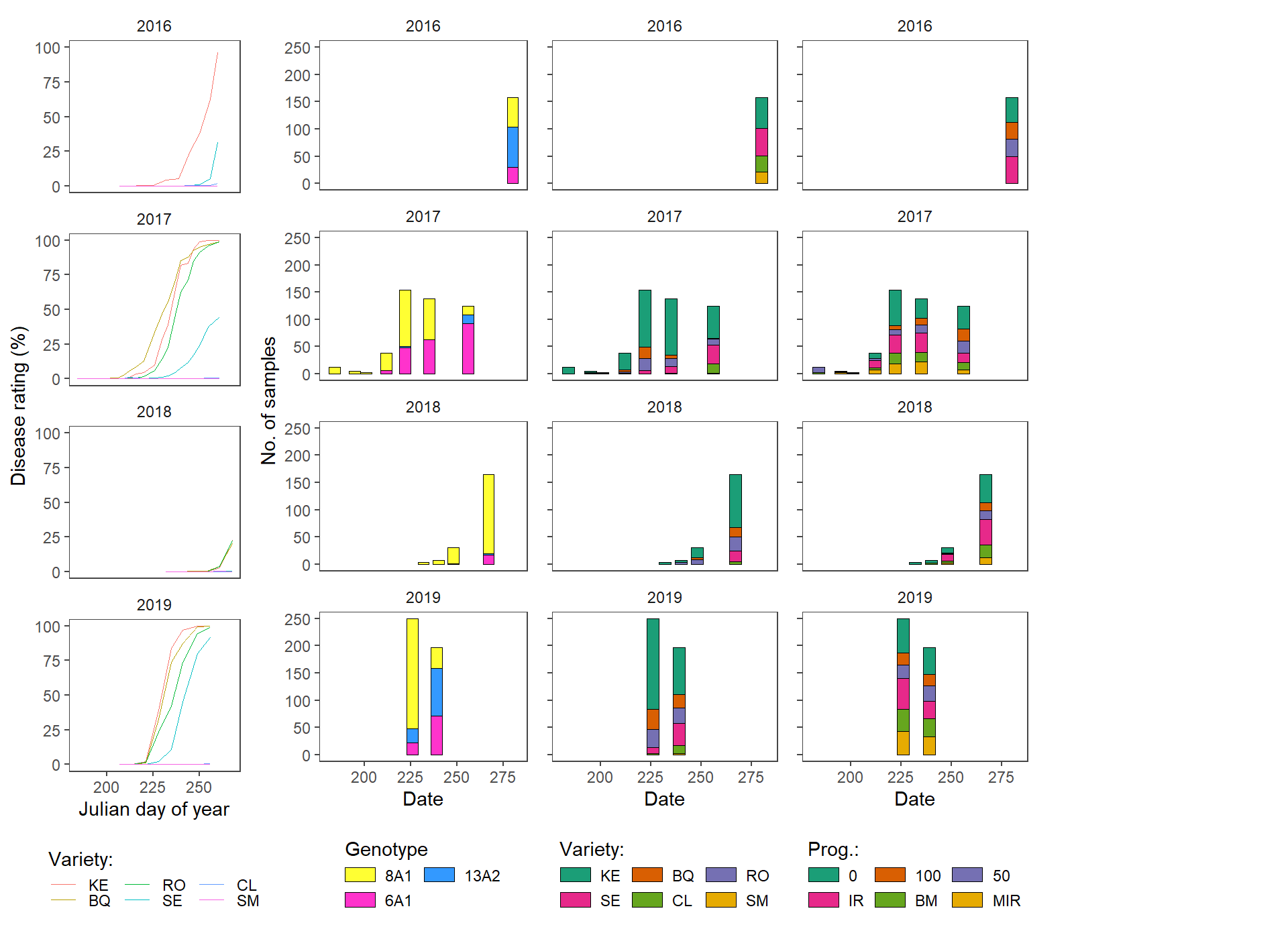
The code
GenPalette <- c ("#ffff33", "#3399ff","#ff33cc")
lab_size <-  3
lab_pos_y <- -0.04

gen_prop <-
  samples %>%
  group_by(variety) %>%
  count(Genotype, variety) %>%
  rename(counts = n) %>%
  mutate(prop = prop.table(counts)) %>%
  mutate(perc = round(prop * 100,1)) %>%
  arrange(desc(variety))


labels <-
  samples %>%
  count( variety) %>%
  rename(counts = n) %>%
  mutate(prop = prop.table(counts)) %>%
  dplyr::select(counts) %>%
  sapply( .,  function(x) paste0("n=", x )) %>%
  as.vector()

f_v <-
  ggplot(gen_prop, aes(variety, prop, fill = Genotype)) +
  geom_hline(
    yintercept = seq(0 , 1, 0.1),
    size = 0.2,
    alpha = 0.8,
    color = "gray",
    linetype = "dotted"
  )+
  geom_bar(stat = "identity",
           width = 0.6,
           position = position_fill(reverse = TRUE),
           color = "black",
           size = .1) +
  ylab("Frequency") +
  xlab("Variety")  +
  annotate(
    geom = "text",
    label = rev(labels),
    x = unique(gen_prop$variety),
    y = lab_pos_y,
    size = lab_size
  )+
  scale_fill_manual(values=GenPalette)+
  theme_bw()+
  egg::theme_article()+
  scale_y_continuous(limits = c(-0.09, 1),
                     # expand = c(0, 0),
                     breaks = seq(0, 1, 0.1))+
  theme(legend.position = "top",
        axis.title.y=element_blank()
  )


gen_prop_trt <-
  samples %>%


  group_by(treatment) %>%
  count(Genotype, treatment) %>%
  rename(counts = n) %>%
  mutate(prop = prop.table(counts))%>%
  mutate(perc = round(prop * 100,1))

labels <-
  samples %>%

  count(treatment) %>%
  rename(counts = n) %>%
  mutate(prop = prop.table(counts)) %>%
  dplyr::select(counts) %>%
  sapply(.,  function(x)
    paste0("n=", x)) %>%
  as.vector()

f_t <-
  ggplot(gen_prop_trt, aes(treatment, prop, fill = Genotype)) +
  geom_hline(
    yintercept = seq(0 , 1, 0.1),
    size = 0.2,
    alpha = 0.8,
    color = "gray",
    linetype = "dotted"
  ) +
  geom_bar(
    stat = "identity",
    width = 0.6,
    position = position_fill(reverse = TRUE),
    color = "black",
    size = .1
  ) +
  ylab("Proportion") +
  xlab("Treatment")  +
  annotate(
    geom = "text",
    label = labels,
    x = unique(gen_prop_trt$treatment),
    y = lab_pos_y,
    size = lab_size
  ) +
  scale_fill_manual(values = GenPalette) +
  egg::theme_article() +
  scale_y_continuous(limits = c(-0.08, 1),
                     # expand = c(0, 0),
                     breaks = seq(0, 1, 0.1)) +
  theme(axis.title.y = element_blank(),
        legend.position = "none")

#Years
gen_prop_year<-
  samples %>%


  group_by(year) %>%
  count(Genotype, year) %>%
  rename(counts = n) %>%
  mutate(prop = prop.table(counts))%>%
  mutate(perc = round(prop * 100,1))

labels <-
  samples %>%
  count( year) %>%
  rename(counts = n) %>%
  mutate(prop = prop.table(counts)) %>%
  dplyr::select(counts) %>%
  sapply( .,  function(x) paste0("n=", x )) %>%
  as.vector()

f_y <-
  ggplot(gen_prop_year, aes(year, prop, fill = Genotype)) +
  geom_hline(
    yintercept = seq(0 , 1, 0.1),
    size = 0.2,
    alpha = 0.8,
    color = "gray",
    linetype = "solid"
  ) +
  geom_bar(
    stat = "identity",
    width = 0.45,
    position = position_fill(reverse = TRUE),
    color = "black",
    size = .1
  ) +
  ylab("Frequency") +
  xlab("Year")  +
  annotate(
    geom = "text",
    label = labels,
    x = unique(gen_prop_year$year),
    y = lab_pos_y,
    size = lab_size
  ) +
  egg::theme_article() +
  scale_y_continuous(
    limits = c(-0.09, 1),
    # expand = c(0, 0),
    breaks = seq(0, 1, 0.1)
  ) +
  scale_fill_manual(values = GenPalette) +
  theme(axis.title.y = element_blank(),
        legend.position = "none")


plotls <- list(f_v, f_t, f_y)

saveRDS(plotls,file = here::here("results", "gen", "freq", "freq_plots.RDS"))


ggpubr::ggarrange(plotlist = plotls,
                  heights = c(1.2,1,1),
                  # labels = c("r","rr"),
                  nrow = 3)+
  ggsave(filename= here::here("results", "gen", "freq", "Freq_all.png"),
         width = 2.9, height =9, dpi = 820)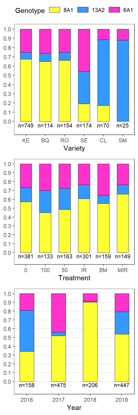
Frequency tables
gen_prop %>%
  dplyr::select(c(variety, Genotype, perc)) %>%
  spread(variety, perc) %>%
  lapply(., replace_na, 0) %>% tbl_df()%>%
kableExtra::kable()| Genotype | KE | BQ | RO | SE | CL | SM |
|---|---|---|---|---|---|---|
| 8A1 | 67.4 | 64.9 | 66.2 | 19.0 | 17.1 | 0 |
| 13A2 | 7.2 | 8.8 | 8.4 | 35.1 | 71.4 | 88 |
| 6A1 | 25.4 | 26.3 | 25.3 | 46.0 | 11.4 | 12 |
gen_prop_trt %>%
  dplyr::select(c(treatment, Genotype, perc)) %>%
  spread(treatment, perc) %>%
kableExtra::kable()| Genotype | 0 | 100 | 50 | IR | BM | MIR |
|---|---|---|---|---|---|---|
| 8A1 | 57.2 | 45.1 | 48.5 | 60.8 | 55.3 | 65.8 |
| 13A2 | 16.0 | 24.8 | 23.9 | 15.6 | 8.8 | 10.7 |
| 6A1 | 26.8 | 30.1 | 27.6 | 23.6 | 35.8 | 23.5 |
gen_prop_year %>%
  dplyr::select(c(year, Genotype, perc)) %>%
  spread(year, perc)  %>%
kableExtra::kable(align = "c")| Genotype | 2016 | 2017 | 2018 | 2019 |
|---|---|---|---|---|
| 8A1 | 34.2 | 51.8 | 90.3 | 53.7 |
| 13A2 | 46.8 | 4.2 | 1.0 | 25.5 |
| 6A1 | 19.0 | 44.0 | 8.7 | 20.8 |
The code
var_gen <-
samples %>%
  filter(year>2016) %>%
  group_by(date) %>%
  count(variety) %>%
  rename(counts = n) %>%
  mutate(prop = prop.table(counts)) %>%
  mutate(perc = round(prop * 100,1)) %>%
  arrange(desc(variety)) %>%
  ungroup()


var_count <-
  var_gen %>%
  dplyr::select(c(date, variety, counts)) %>%
  spread(variety, counts)

var_count[ ,-1] <-
var_count[ ,-1] %>%
  lapply(., replace_na, 0) %>% tbl_df()

var_count <-
var_count%>%
  mutate(Sus = KE + BQ+ RO,
         Med = SE,
         Res = CL + SM)

var_prop <-
  var_gen %>%
  dplyr::select(c(date, variety, perc)) %>%
  spread(variety, perc)

var_prop[, -1] <-
  var_prop[, -1] %>%
  lapply(., replace_na, 0) %>% tbl_df()

var_prop <-
  var_prop%>%
  mutate(Sus = KE + BQ+ RO,
         Med = SE,
         Res = CL + SM)

for (i in seq(colnames(var_prop[,-1]))) {
  vec <- var_count[, i + 1] %>% pull %>% as.character() %>% as.list()
  vec_prop <-
    var_prop[, i + 1] %>% pull %>% as.character() %>% as.list()

  newvec <- vector()
  for (y in seq(vec)) {
    newvec[y] <- paste0(vec[y], " (", vec_prop[y], ")")
  }

  var_count[, i + 1] <- newvec
}

write.csv(var_count, file = here::here("results", "gen", "Samples per variety par sampling date.csv"))
var_count%>%
kableExtra::kable(align = "c")| date | KE | BQ | RO | SE | CL | SM | Sus | Med | Res |
|---|---|---|---|---|---|---|---|---|---|
| 2017-07-03 | 12 (100) | 0 (0) | 0 (0) | 0 (0) | 0 (0) | 0 (0) | 12 (100) | 0 (0) | 0 (0) |
| 2017-07-14 | 3 (60) | 1 (20) | 1 (20) | 0 (0) | 0 (0) | 0 (0) | 5 (100) | 0 (0) | 0 (0) |
| 2017-07-20 | 1 (33.3) | 1 (33.3) | 1 (33.3) | 0 (0) | 0 (0) | 0 (0) | 3 (99.9) | 0 (0) | 0 (0) |
| 2017-07-31 | 30 (78.9) | 4 (10.5) | 3 (7.9) | 1 (2.6) | 0 (0) | 0 (0) | 37 (97.3) | 1 (2.6) | 0 (0) |
| 2017-08-10 | 105 (68.2) | 20 (13) | 23 (14.9) | 6 (3.9) | 0 (0) | 0 (0) | 148 (96.1) | 6 (3.9) | 0 (0) |
| 2017-08-23 | 104 (75.4) | 5 (3.6) | 15 (10.9) | 13 (9.4) | 0 (0) | 1 (0.7) | 124 (89.9) | 13 (9.4) | 1 (0.7) |
| 2017-09-13 | 60 (48) | 1 (0.8) | 11 (8.8) | 34 (27.2) | 18 (14.4) | 1 (0.8) | 72 (57.6) | 34 (27.2) | 19 (15.2) |
| 2018-08-20 | 3 (100) | 0 (0) | 0 (0) | 0 (0) | 0 (0) | 0 (0) | 3 (100) | 0 (0) | 0 (0) |
| 2018-08-28 | 4 (57.1) | 0 (0) | 3 (42.9) | 0 (0) | 0 (0) | 0 (0) | 7 (100) | 0 (0) | 0 (0) |
| 2018-09-05 | 19 (61.3) | 4 (12.9) | 8 (25.8) | 0 (0) | 0 (0) | 0 (0) | 31 (100) | 0 (0) | 0 (0) |
| 2018-09-24 | 97 (58.8) | 18 (10.9) | 26 (15.8) | 19 (11.5) | 5 (3) | 0 (0) | 141 (85.5) | 19 (11.5) | 5 (3) |
| 2019-08-14 | 167 (66.8) | 36 (14.4) | 34 (13.6) | 11 (4.4) | 2 (0.8) | 0 (0) | 237 (94.8) | 11 (4.4) | 2 (0.8) |
| 2019-08-27 | 87 (44.2) | 24 (12.2) | 29 (14.7) | 40 (20.3) | 15 (7.6) | 2 (1) | 140 (71.1) | 40 (20.3) | 17 (8.6) |
Temporal structure
Proportion og MLG per sampling date.
The code
dis_obs <-
  filter(dis_obs, year != 2016)

########################################
#sus
#####################################################


sdf <-
samples %>%
  dplyr::filter( variety %in% c("KE", "BQ","RO" )) %>%
  dplyr::filter( treatment %in% c( "IR","0")) %>%
  dplyr::filter( year != 2016)

temporal_prop_sus <-
sdf %>%
  group_by(date) %>%
  count(Genotype) %>%
  rename(counts = n) %>%
  mutate(prop = prop.table(counts)) %>%
  mutate(perc = round(prop * 100,1)) %>%
  select(date, Genotype, perc) %>%
  spread(., Genotype, perc) %>%
  replace(is.na(.), 0) %>%
  arrange(date) %>%
  add_column( ., Year = format(.$date, "%Y"), .before= "date") %>%
  mutate("13A2+6A1 (%)" = `13A2` + `6A1`) %>%
  rename("8A1 (%)" = "8A1",
         "6A1 (%)" = "6A1",
         "13A2 (%)" = "13A2",
         "Sampling Date" = "date")


counts_df_sus <-
sdf%>%
  group_by(date)%>%
  count(counts =n())

temporal_prop_sus <-
  add_column( temporal_prop_sus, `No. of Samples` =counts_df_sus$counts, .before= "8A1 (%)")


write_csv(temporal_prop_sus, here::here("results", "gen", "MLG per date sus.csv"))


counts_df_sus$labels <-
  sapply(counts_df_sus[["counts"]],  function(x) paste0("n=", x )) %>%
  as.vector()

sdf <-
left_join(sdf, counts_df_sus, by = c("date")) %>%
  mutate(set = "Subset")

########################################
#all
#####################################################


adf <-
  samples %>%
  # dplyr::filter( variety %in% c("KE", "BQ","RO" )) %>%
  dplyr::filter( year != 2016)

temporal_prop <-
  adf %>%
  group_by(date) %>%
  count(Genotype) %>%
  rename(counts = n) %>%
  mutate(prop = prop.table(counts)) %>%
  mutate(perc = round(prop * 100,1)) %>%
  select(date, Genotype, perc) %>%
  spread(., Genotype, perc) %>%
  replace(is.na(.), 0) %>%
  arrange(date) %>%
  add_column( ., Year = format(.$date, "%Y"), .before= "date") %>%
  mutate("13A2+6A1 (%)" = `13A2` + `6A1`) %>%
  rename("8A1 (%)" = "8A1",
         "6A1 (%)" = "6A1",
         "13A2 (%)" = "13A2",
         "Sampling Date" = "date")


counts_df <-
  adf%>%
  dplyr::filter( year != 2016) %>%
  group_by(date)%>%
  count(counts =n())

temporal_prop <-
  add_column( temporal_prop, `No. of Samples` =counts_df$counts, .before= "8A1 (%)")


write_csv(temporal_prop, here::here("results", "gen", "MLG per date.csv"))


counts_df$labels <-
  sapply(counts_df[["counts"]],  function(x) paste0("n=", x )) %>%
  as.vector()

adf <-
  left_join(adf, counts_df, by = c("date")) %>%
  mutate(set = "All Samples")

#####################################################
#plot
#####################################################


samples_fig <-
   bind_rows( adf, sdf)


cbbPalette <- c ( "#ffff33","#3399ff", "#ff33cc")

dis_obs <-
  dplyr::filter(dis_obs, treatment == "Control") %>%
  mutate(treatment = "Control plots") %>%
  group_by(treatment, variety, year, julian_day) %>%
  summarise(rating = mean(obs))

ptemp <-
ggplot() +
  geom_bar(
    data = samples_fig,
    aes(julian_day, fill = Genotype),
    stat = "count",
    position = "fill",
    width = 4.7,
    colour = "black",
    size = line_size
  ) +
  geom_line(
    data = dis_obs,
    aes(
      x = as.numeric(julian_day),
      y = rating / 100,
      colour = variety,
      group = variety
    ),
    size = .4,
    alpha = .6,
    linetype = "solid"
  ) +
  facet_grid( year~ set  ) +
  xlab("Day of year")+
  ylab("Proportion of foliar disease and MLGs")+
  scale_y_continuous(limits = c(-0.132, 1),
                     breaks = seq(0, 1, 0.2)) +
  scale_fill_manual(values=cbbPalette)+
  theme_article()+
  labs(fill = "MLG:",
       color = "Variety")+
  scale_colour_brewer("Variety:",
                      palette = "Dark2")+
  # ## Uncomment for vertical plot
    # geom_text(data = samples_fig,
    #         aes(x = julian_day, y = -0.07, label = labels),
    #         size = 2.2,
    #         check_overlap = FALSE) +

  # theme( legend.position = "bottom",
  #        legend.direction = "horizontal")+
  # guides(fill=guide_legend(nrow=1,byrow=TRUE,title.position = "top"),
  #        color=guide_legend(nrow=2,byrow=TRUE,title.position = "top"))+
  # ggsave(filename= here::here("results", "gen", "freq", "Genotype and DPC per sampling vertical.png"),
  #        width = 5, height =7, dpi = 620)
  # Uncomment for horisontal plot
   facet_grid( set~ year  ) +
  geom_text(data = samples_fig,
            aes(x = julian_day, y = -0.1, label = labels),
            size = 3.4,
            angle = -40) +
  guides(fill=guide_legend(nrow=1,byrow=TRUE,title.position = "top"),
         color=guide_legend(nrow=1,byrow=TRUE,title.position = "top"))+
  theme(text = element_text(size = 15),
        legend.position = "bottom")

ptemp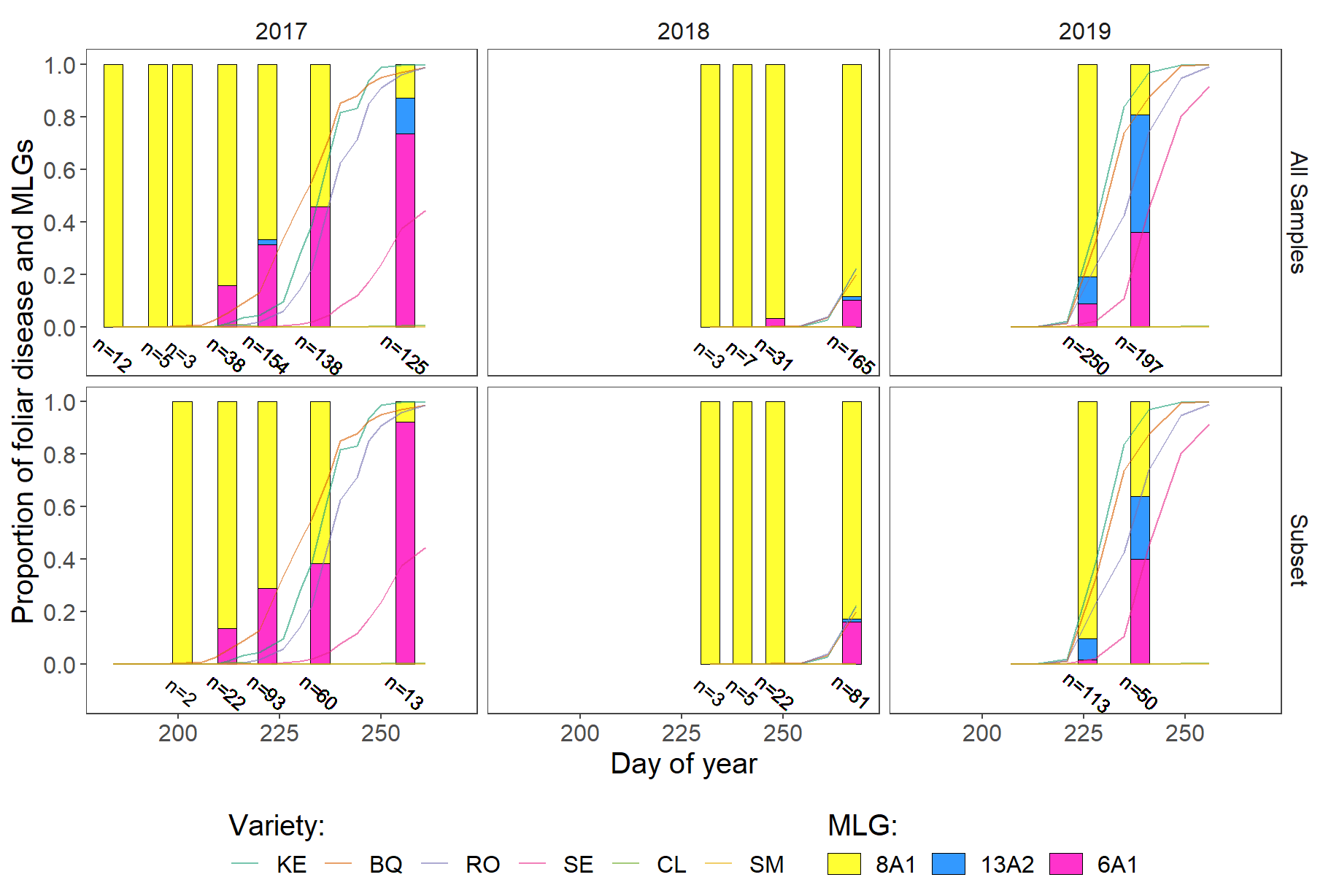
The code
  ggsave(plot = ptemp,
         filename= here::here("results", "gen", "freq", "Genotype and DPC per sampling horisontal.png"),
width = 10, height =6.5, dpi = 620)session_info()## - Session info ----------------------------------------------------------
## setting value
## version R version 3.6.3 (2020-02-29)
## os Windows 10 x64
## system x86_64, mingw32
## ui RTerm
## language (EN)
## collate English_United States.1252
## ctype English_United States.1252
## tz Europe/London
## date 2020-08-17
##
## - Packages --------------------------------------------------------------
## package * version date lib source
## assertthat 0.2.1 2019-03-21 [1] CRAN (R 3.6.1)
## backports 1.1.5 2019-10-02 [1] CRAN (R 3.6.1)
## broom 0.5.5 2020-02-29 [1] CRAN (R 3.6.3)
## callr 3.4.2 2020-02-12 [1] CRAN (R 3.6.3)
## cellranger 1.1.0 2016-07-27 [1] CRAN (R 3.6.1)
## cli 2.0.2 2020-02-28 [1] CRAN (R 3.6.3)
## colorspace 1.4-1 2019-03-18 [1] CRAN (R 3.6.1)
## conflicted * 1.0.4 2019-06-21 [1] CRAN (R 3.6.1)
## cowplot 1.0.0 2019-07-11 [1] CRAN (R 3.6.1)
## crayon 1.3.4 2017-09-16 [1] CRAN (R 3.6.1)
## DBI 1.1.0 2019-12-15 [1] CRAN (R 3.6.3)
## dbplyr 1.4.2 2019-06-17 [1] CRAN (R 3.6.1)
## desc 1.2.0 2018-05-01 [1] CRAN (R 3.6.1)
## devtools * 2.2.2 2020-02-17 [1] CRAN (R 3.6.3)
## digest 0.6.25 2020-02-23 [1] CRAN (R 3.6.3)
## dplyr * 0.8.5 2020-03-07 [1] CRAN (R 3.6.3)
## egg * 0.4.5 2019-07-13 [1] CRAN (R 3.6.1)
## ellipsis 0.3.0 2019-09-20 [1] CRAN (R 3.6.1)
## evaluate 0.14 2019-05-28 [1] CRAN (R 3.6.1)
## fansi 0.4.1 2020-01-08 [1] CRAN (R 3.6.3)
## farver 2.0.3 2020-01-16 [1] CRAN (R 3.6.3)
## forcats * 0.4.0 2019-02-17 [1] CRAN (R 3.6.1)
## fs 1.3.1 2019-05-06 [1] CRAN (R 3.6.1)
## generics 0.0.2 2018-11-29 [1] CRAN (R 3.6.1)
## ggplot2 * 3.3.1 2020-05-28 [1] CRAN (R 3.6.3)
## ggpubr 0.2.4 2019-11-14 [1] CRAN (R 3.6.2)
## ggsignif 0.6.0 2019-08-08 [1] CRAN (R 3.6.1)
## glue 1.4.0 2020-04-03 [1] CRAN (R 3.6.3)
## gridExtra * 2.3 2017-09-09 [1] CRAN (R 3.6.1)
## gtable 0.3.0 2019-03-25 [1] CRAN (R 3.6.1)
## haven 2.3.0 2020-05-24 [1] CRAN (R 3.6.3)
## here 0.1 2017-05-28 [1] CRAN (R 3.6.1)
## highr 0.8 2019-03-20 [1] CRAN (R 3.6.1)
## hms 0.5.2 2019-10-30 [1] CRAN (R 3.6.1)
## htmltools 0.4.0 2019-10-04 [1] CRAN (R 3.6.1)
## httr 1.4.1 2019-08-05 [1] CRAN (R 3.6.1)
## jsonlite 1.6.1 2020-02-02 [1] CRAN (R 3.6.3)
## kableExtra * 1.1.0 2019-03-16 [1] CRAN (R 3.6.1)
## knitr 1.25 2019-09-18 [1] CRAN (R 3.6.1)
## labeling 0.3 2014-08-23 [1] CRAN (R 3.6.0)
## lattice 0.20-38 2018-11-04 [2] CRAN (R 3.6.3)
## lifecycle 0.2.0 2020-03-06 [1] CRAN (R 3.6.3)
## lubridate 1.7.4 2018-04-11 [1] CRAN (R 3.6.1)
## magrittr 1.5 2014-11-22 [1] CRAN (R 3.6.1)
## memoise 1.1.0 2017-04-21 [1] CRAN (R 3.6.1)
## modelr 0.1.5 2019-08-08 [1] CRAN (R 3.6.1)
## munsell 0.5.0 2018-06-12 [1] CRAN (R 3.6.1)
## nlme 3.1-144 2020-02-06 [2] CRAN (R 3.6.3)
## pillar 1.4.3 2019-12-20 [1] CRAN (R 3.6.3)
## pkgbuild 1.0.6 2019-10-09 [1] CRAN (R 3.6.1)
## pkgconfig 2.0.3 2019-09-22 [1] CRAN (R 3.6.1)
## pkgload 1.0.2 2018-10-29 [1] CRAN (R 3.6.1)
## prettyunits 1.0.2 2015-07-13 [1] CRAN (R 3.6.1)
## processx 3.4.1 2019-07-18 [1] CRAN (R 3.6.1)
## ps 1.3.0 2018-12-21 [1] CRAN (R 3.6.1)
## purrr * 0.3.3 2019-10-18 [1] CRAN (R 3.6.1)
## R6 2.4.1 2019-11-12 [1] CRAN (R 3.6.3)
## RColorBrewer 1.1-2 2014-12-07 [1] CRAN (R 3.6.0)
## Rcpp 1.0.4.6 2020-04-09 [1] CRAN (R 3.6.3)
## readr * 1.3.1 2018-12-21 [1] CRAN (R 3.6.1)
## readxl 1.3.1 2019-03-13 [1] CRAN (R 3.6.1)
## remotes 2.1.1 2020-02-15 [1] CRAN (R 3.6.3)
## reprex 0.3.0 2019-05-16 [1] CRAN (R 3.6.1)
## rlang 0.4.5 2020-03-01 [1] CRAN (R 3.6.3)
## rmarkdown 2.1 2020-01-20 [1] CRAN (R 3.6.3)
## rprojroot 1.3-2 2018-01-03 [1] CRAN (R 3.6.1)
## rstudioapi 0.11 2020-02-07 [1] CRAN (R 3.6.3)
## rvest 0.3.5 2019-11-08 [1] CRAN (R 3.6.3)
## scales 1.1.0 2019-11-18 [1] CRAN (R 3.6.3)
## sessioninfo 1.1.1 2018-11-05 [1] CRAN (R 3.6.1)
## stringi 1.4.6 2020-02-17 [1] CRAN (R 3.6.2)
## stringr * 1.4.0 2019-02-10 [1] CRAN (R 3.6.1)
## tableHTML * 2.0.0 2019-03-16 [1] CRAN (R 3.6.1)
## testthat 2.2.1 2019-07-25 [1] CRAN (R 3.6.1)
## tibble * 3.0.0 2020-03-30 [1] CRAN (R 3.6.3)
## tidyr * 1.0.0 2019-09-11 [1] CRAN (R 3.6.1)
## tidyselect 1.0.0 2020-01-27 [1] CRAN (R 3.6.3)
## tidyverse * 1.3.0 2019-11-21 [1] CRAN (R 3.6.3)
## usethis * 1.5.1 2019-07-04 [1] CRAN (R 3.6.1)
## vctrs 0.3.0 2020-05-11 [1] CRAN (R 3.6.3)
## viridisLite 0.3.0 2018-02-01 [1] CRAN (R 3.6.1)
## webshot 0.5.1 2018-09-28 [1] CRAN (R 3.6.1)
## withr 2.1.2 2018-03-15 [1] CRAN (R 3.6.1)
## xfun 0.10 2019-10-01 [1] CRAN (R 3.6.1)
## xml2 1.3.2 2020-04-23 [1] CRAN (R 3.6.3)
## yaml 2.2.0 2018-07-25 [1] CRAN (R 3.6.0)
##
## [1] C:/Users/mlade/Documents/R/win-library/3.6
## [2] C:/Program Files/R/R-3.6.3/library