Analysis
Here I present the model and the methodology used in the analysis.
Libraries
Packages needed for the analysis are loaded. If the libraries do not exist locally, they will be downloaded.
list.of.packages <-
  c(
    "tidyverse",
    "readxl",
    "ggrepel",
    "pracma",
    "remotes",
    "parallel",
    "pbapply",
    "R.utils",
    "rcompanion",
    "mgsub",
    "here",
    "stringr",
    "pander",
    "tools",
    "kableExtra"
  )

new.packages <-
  list.of.packages[!(list.of.packages %in% installed.packages()[, "Package"])]

#Download packages that are not already present
if (length(new.packages))
  install.packages(new.packages)

if ("gt" %in% installed.packages() == FALSE)
  remotes::install_github("rstudio/gt")

list.of.packages <- c(list.of.packages, "gt")
packages_load <-
  lapply(list.of.packages, require, character.only = TRUE)

#Print warning if there is a problem with installing/loading some of packages
if (any(as.numeric(packages_load) == 0)) {
  warning(paste("Package/s: ", paste(list.of.packages[packages_load != TRUE], sep = ", "), "not loaded!"))
} else {
  print("All packages were successfully loaded.")
}
## [1] "All packages were successfully loaded."rm(list.of.packages, new.packages, packages_load)The Model
According to the Irish Rules (Bourke, 1953), temperatures ≥ 10 ℃ and relative humidity ≥ 90 % provide the necessary environmental conditions considered conducive for potato late blight. The blight epidemic onset risk is then estimated during periods fulfilling the following criteria:
* Sporulation period is the initial stage considered necessary for the formation of sporangia is set to a minimum of 12 consecutive hours and is referred to as the sporulation duration threshold (SDt) in this evaluation;
* Infection period starts after the sporulation period and is reduced by 4 hours if the surface of plants was not wet at the beginning of the infection period. The leaf (surface) wetness is considered present if there was a considerable amount of precipitation (≥ 0.1 mm) during the time window of 3 hours before and 3 hours after the 12th consecutive hour of sporulation. The infection period lasts until conditions are not broken for more than 5h (spore survival).
Implementation of the model.
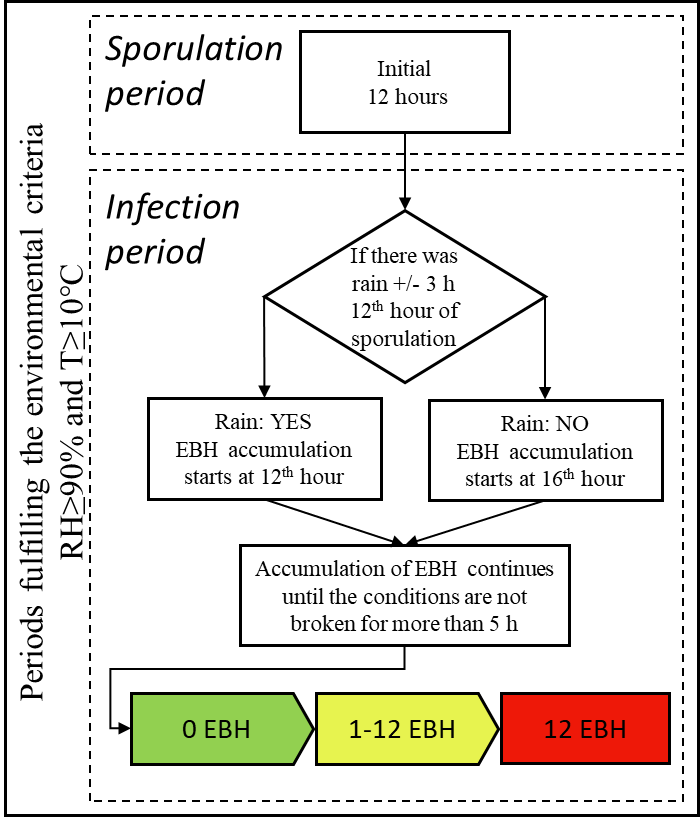
Irish Rules simplified alghorithm schematics.
The code
IrishRulesModel <- function(weather,
                            param = NULL,
                            infill_gap = NULL) {
#' Irish Rules
#'
#' This function calculates potatolate blight risk using Irish Rules model (Bourke, 1953)
#' @param weather The weather data in formated as data frame
#' @param infill_gap Maximum alowed gap for missing value interpolation
#' @keywords Irish Rules
#'
  # wetness requirement prior to infection accumulation start
  # time window of 6 hours, 3 before/after sporulation ends
  wet_before <- 3
  wet_after <- 3

  # Parameter list
  if (is.null(param)) {
    rh_thresh <- 90
    temp_thresh <- 10
    hours <- 12   #sum of hours before EBH accumulation
  } else {
    #pass a vector of parameters
    rh_thresh <- as.numeric(param[2])
    temp_thresh <- as.numeric(param[3])
    hours <- as.numeric(param[4])
    lw_rhum <-
      param[5]           #if is NA then only rain data will be used
  }

  #threshold for estimation of leaf wetness using relative humidity
  lw_rhum_threshold <- 90

  weather[["rain"]] -> rain
  if ("rhum" %in% names(weather)) {
    weather[["rhum"]] -> rh
  }
  if ("rh" %in% names(weather)) {
    weather[["rh"]] -> rh
  }
  weather[["temp"]] -> temp

  # This function to infil missing values to let the model run
  #If maximum infill gap is not provided it is defaulted to 7
  if (is.null(infill_gap)) {
    infill_gap <- 7
  }

  if (sum(is.na(with(weather, rain, temp, rhum))) > 0) {
    temp <-
      round(zoo::na.spline(temp, na.rm = FALSE, maxgap = infill_gap), 1)
    rh <-
      round(zoo::na.spline(rh, na.rm = FALSE, maxgap = infill_gap), 0)
    rh  <- sapply(rh, function(x) ifelse(x > 100, x <- 100, x))
  }

  if (sum(is.na(with(weather, rain, temp, rhum))) > 0) {
    stop(print("The sum of NAs is more than 7! Check your weather data."))
  }

  # "Out of boounds"
  rain <- c(rain, rep(0, 20))
  temp <- c(temp, rep(0, 20))
  rh <- c(rh, rep(0, 20))

  # conditions for sporulation
  criteria <- as.numeric(temp >= temp_thresh & rh >= rh_thresh)

  # cumulative sum of hours that meet the criteria for sporulatoion with restart at zero
  criteria_sum <-
    stats::ave(criteria, cumsum(criteria == 0), FUN = cumsum)

  # Initiate risk accumulation vector
  risk <- rep(0, length(temp))

  criteria_met12  <-
    as.numeric(criteria_sum >= hours) #accumulation of EBH starts after sporulation
  idx             <- which(criteria_sum == hours)

  #If there are no accumulations return vector with zeros
  if (sum(criteria_sum == hours) == 0) {
    #breaks the loop if there is no initial accumulation of 12 hours
    head(risk, -20)
  } else{
    for (j in 1:length(idx)) {
      #switch that looks if there was wetness: first rain, then both rain and rh, if rh exists
      if (if (lw_rhum == "rain") {
        #if only rain
        (sum(rain[(idx[j] - wet_before):(idx[j] + wet_after)]) >= 0.1)           #just see rain sum
      } else{
        any((any(rh[(idx[j] - wet_before):(idx[j] + wet_after)] >= lw_rhum_threshold)) |
            #take both as possible switches
            (sum(rain[(idx[j] - wet_before):(idx[j] + wet_after)]) >= 0.1))
      })
        # outputs true or false
      {
        n <- idx[j]        #start accumulation from 12th hour
      } else {
        n <- idx[j] + 4      #start accumulation from 16th hour
      }
      s <- criteria_met12[n]

      # if a break of less than or equal to 5 hours
      m <- n - 1

      while (s == 1)
      {
        risk[n] <- risk[m] + 1
        n <- n + 1
        m <- n - 1
        s <- criteria[n]
        if (s == 0 && (criteria[n + 2] == 1)) {
          n = n + 2
          s = 1
        } else if (s == 0 && (criteria[n + 3] == 1)) {
          n = n + 3
          s = 1
        } else if (s == 0 && (criteria[n + 4] == 1)) {
          n = n + 4
          s = 1
        } else if (s == 0 && (criteria[n + 5] == 1)) {
          n = n + 5
          s = 1
        }
      }

    }
    head(risk, -20) #remove last 20 values that were added to vectors to prevent "Out of bounds" issue
  }
}
Bio dates
Emergence takes around 3 weeks under Irish conditions. Period when healthy host present is considered to last from emergence until 14 days prior to the first observation of the disease in the field. A 10-day ‘warning period’ considered to last from -14 days to – 4 days prior to disease observed in the field. The 4-day period was assumed to be a minimum time needed from incubation period, for the establishment of visible disease symptoms in the field.
#Get subsets of data for period before the epidemics were initiated
dates_cut <-
  read_csv(
    here::here("data", "op_2007_16", "raw", "plantingdates.csv"),
    col_types = cols(
      disease_observed = col_date(format = "%d/%m/%Y"),
      planting_date =  col_date(format = "%d/%m/%Y")
    )
  )


dates_cut <-
  add_column(dates_cut,
             emergence = as.Date(dates_cut$planting_date) + 21,
             .before = "planting_date")
#set warnning period to 14 days before disease onset
dates_cut <- add_column(dates_cut, disease_onset = as.Date(dates_cut$disease_observed) - 4,
                        .before = "disease_observed")

dates_cut <- add_column(dates_cut, warning = as.Date(dates_cut$disease_onset) - 10, .before = "disease_onset" )
rownames(dates_cut) <- NULL

dates_cut %>%
  rename_all(. %>%
               gsub("_", " ", .) %>%
               tools::toTitleCase()) %>%
  kable(format = "html") %>%
kableExtra::kable_styling( latex_options = "striped",full_width = FALSE)| Year | Emergence | Planting Date | Warning | Disease Onset | Disease Observed |
|---|---|---|---|---|---|
| 2007 | 2007-04-24 | 2007-04-03 | 2007-06-16 | 2007-06-26 | 2007-06-30 |
| 2008 | 2008-04-28 | 2008-04-07 | 2008-06-18 | 2008-06-28 | 2008-07-02 |
| 2009 | 2009-05-12 | 2009-04-21 | 2009-06-22 | 2009-07-02 | 2009-07-06 |
| 2010 | 2010-05-25 | 2010-05-04 | 2010-07-05 | 2010-07-15 | 2010-07-19 |
| 2011 | 2011-05-27 | 2011-05-06 | 2011-07-14 | 2011-07-24 | 2011-07-28 |
| 2012 | 2012-06-18 | 2012-05-28 | 2012-06-29 | 2012-07-09 | 2012-07-13 |
| 2013 | 2013-06-24 | 2013-06-03 | 2013-08-09 | 2013-08-19 | 2013-08-23 |
| 2014 | 2014-06-13 | 2014-05-23 | 2014-07-18 | 2014-07-28 | 2014-08-01 |
| 2015 | 2015-06-12 | 2015-05-22 | 2015-07-17 | 2015-07-27 | 2015-07-31 |
| 2016 | 2016-06-21 | 2016-05-31 | 2016-07-08 | 2016-07-18 | 2016-07-22 |
The Analysis
The set of the most important variables of Irish rules model is evaluated. The Excel sheet with parameters under evaluation is available in data folder and can be changed and used for model evaluation in other locations. Column named 90_10_12_rain represents set of the original model parameters.
#read in parameters
parameters <-
  read_excel(here::here("data", "op_2007_16", "raw", "par.xlsx"), sheet = "par")
parameters
params <- expand.grid(parameters[, 1:3])
#set the leaf wetness threshold to NA, meaning only rain is considered as an estimator for leaf wetness, as in original model
params$lw_rh <- "rain"
#Repeat all of the analysis considering rh >= 90% and rain as an estimator of leaf wetness
params2 <- params
params2$lw_rh <- as.character("rainrh")
parameters <- bind_rows(params, params2)
rm(params, params2)
# set a column with a name for each model
parameters <- add_column(parameters, model = NA, .before = 1)
for (i in seq_along(1:nrow(parameters))) {
parameters[i, 1] <-
paste0(parameters[i, 2:length(names(parameters))], collapse = "_")
}
str(parameters)## 'data.frame': 686 obs. of 5 variables:
## $ model : chr "93_13_15_rain" "92_13_15_rain" "91_13_15_rain" "90_13_15_rain" ...
## $ rh_thresh : num 93 92 91 90 89 88 87 93 92 91 ...
## $ temp_thresh: num 13 13 13 13 13 13 13 12 12 12 ...
## $ hours : num 15 15 15 15 15 15 15 15 15 15 ...
## $ lw_rh : chr "rain" "rain" "rain" "rain" ...Model Run
The model has been run with each set of parameters, and columns with model outputs are attached to weather data frame. Names of new columns correspond to the set of parameters supplied.
# This chunk is not run
load(OP, file = here::here("data", "op_2007_16",  "OP_2007-2016_infilled.RData"))

for(i in 1:nrow(parameters)) {
  loop_var <- apply(parameters[i, ], 1, function(x) {
    #run the model with different parameters
    k <-
      lapply(split(OP, factor(OP$year)), function(chunk)
        IrishRulesModel(chunk, x)) #get the list of outputs
    unlist(k) -> k  #make it a vector
  })
  #attach each output of each model version to the data
  OP[, ncol(OP) + 1] <-  as.numeric(loop_var)
  rm(loop_var)
  names(OP)[ncol(OP)] <- paste0(parameters[i, 1])
  print(paste(i, "of", nrow(parameters)))
}


nn <- paste0(names(OP[, 26:length(names(OP))]), "_ebh", "")
setnames(OP, old = c(names(OP[, 26:length(names(OP))])), new = nn)
rm( nn)
Instead, just load the output from a prior model run to save time.
load(file = here::here("data", "op_2007_16", "OP_for_analysis.RData"))
# Sample of outputs
head(OP[, c(1, 7, 9, 15, 24:30)], 5) %>%
  kable() %>%
kableExtra::kable_styling(latex_options = "striped",full_width = FALSE)| date | doy | rain | vappr | stna | sol_rad | 93_13_15_rain_ebh | 92_13_15_rain_ebh | 91_13_15_rain_ebh | 90_13_15_rain_ebh | 89_13_15_rain_ebh | |
|---|---|---|---|---|---|---|---|---|---|---|---|
| 2401162 | 2007-04-01 00:00:00 | 91 | 0 | 8.0 | Oak_Park | 0 | 0 | 0 | 0 | 0 | 0 |
| 2401163 | 2007-04-01 01:00:00 | 91 | 0 | 7.9 | Oak_Park | 0 | 0 | 0 | 0 | 0 | 0 |
| 2401164 | 2007-04-01 02:00:00 | 91 | 0 | 7.9 | Oak_Park | 0 | 0 | 0 | 0 | 0 | 0 |
| 2401165 | 2007-04-01 03:00:00 | 91 | 0 | 7.6 | Oak_Park | 0 | 0 | 0 | 0 | 0 | 0 |
| 2401166 | 2007-04-01 04:00:00 | 91 | 0 | 7.2 | Oak_Park | 0 | 0 | 0 | 0 | 0 | 0 |
Evaluation Procedure
The function SensParametersCalc calculates Sensitivity and Specificity of each variation of the model.
The code
SensParametersCalc <-
  function(y,
           weather_data,
           dates_cut,
           prot_duration = NULL) {
#' Sensitivity analysis
#'
#' The function `SensParametersCalc` calculates Sensitivity and Specificity of each variation of the model.
#' @param y Decision threeshold (EBH).
#' @param weather_data The weather data  formated as a data frame, containing outputs of all model runs with different parameters.
#' @param dates_cut Dates defining the the periods of evaulation. Specificity is calculated for the period from planting date to warning date. Sensitivity is calculated for the period from -14 to -4 days before the disease is observed in the field.
#' @param prot_duration Each time the warning threshold is reached during the period from planting date to warning date, one treatment is assumed, which would provide protedtion for indicated number of days.
#'

    #Set the warning threshold and run the rest of the script
    warning_threshold <- y
    #data
    fun_df <- weather_data

    #A function to subset the data for the period of interest in each year
    test.overlap = function(vals, start_date, end_date) {
      rowSums(mapply(function(a, b)
        between(vals, a, b),
        start_date, end_date)) > 0
    }

    #Subset  each year from emergence to disease onset and calculate number of FP and TN
    fptn_df <-
      fun_df  %>%
      #Subset the of the data for the duration of non-warning period for each year
      filter(test.overlap(short_date, dates_cut$emergence, dates_cut$warning)) %>%
      select(
        ends_with("year_var"),
        ends_with("week_var"),
        ends_with("doy"),
        ends_with("_ebh")
      ) %>%
      group_by(year_var) %>%
      #if there was an accumulation from previous day, it would triger a warning
      #Check all of the first five rows because of possible break of 5 hours
      mutate_at(., .vars = colnames(.[grep("ebh", colnames(.))]),
                funs(
                  ifelse(row_number() <= 5 & . >= warning_threshold,
                         warning_threshold, .)
                )) %>%
      #all five values all changed so we have to delete 4 of them and leave only 1
      mutate_at(., .vars = colnames(.[grep("ebh", colnames(.))]),
                funs(ifelse(
                  row_number() <= 4 & . == warning_threshold, 0, .
                ))) %>%
      # Change values coresponding to the warning threshold to 1 for calculating the sum
      mutate_at(., .vars = colnames(.[grep("ebh", colnames(.))]),
                funs(ifelse(. == warning_threshold, 1, 0))) %>%
      group_by(year_var, week_var, doy) %>%
      summarise_at(., .vars = colnames(.[grep("ebh", colnames(.))]), .funs = sum)


    #Each warning would cause treatment that will keep the plants protected for a period of time
    prot_duration <-
      ifelse(is.null(prot_duration), 7, prot_duration)#If not defined default value is 7 days

    TreatmentWindow <- function(x, prot_duration) {
      y <-
        vector(mode = "numeric", length = length(x) + prot_duration)
      for (i in seq_along(x)) {
        if (x[i] == 1) {
          y[i:c(i + prot_duration)] <- 1
        }
      }
      y
    }
    fptn_df[grep("ebh", colnames(fptn_df))] <-
      lapply(fptn_df[grep("ebh", colnames(fptn_df))], function(x)
        TreatmentWindow(x, prot_duration))


    FP <-
      summarise_all(fptn_df[, colnames(fptn_df[, grep("ebh", colnames(fptn_df))])], .funs = sum)

    #Each warning will cause a treatment
    total_days <-
      nrow(fptn_df) #total  duration of non_warning period

    TN <- total_days - FP


    ##########################################################
    #subset for 10 days prior to disease onset: Warning period
    tpfn_df <-
      fun_df %>%
      #Subset of the data for the duration WARNING period in each year
      filter(test.overlap(short_date,  dates_cut$warning, dates_cut$disease_onset)) %>%
      select(
        ends_with("year_var"),
        ends_with("week_var"),
        ends_with("doy"),
        ends_with("_ebh")
      ) %>%
      mutate_at(., .vars = colnames(.[grep("ebh", colnames(.))]),
                funs(
                  ifelse(row_number() <= 5 &
                           . >= warning_threshold, warning_threshold, .)
                )) %>%
      #all five values is changed so we have to delete 4 of them and leave only one
      mutate_at(., .vars = colnames(.[grep("ebh", colnames(.))]),
                funs(ifelse(
                  row_number() <= 4 & . == warning_threshold,
                  0, .
                ))) %>%
      mutate_at(., .vars = colnames(.[grep("ebh", colnames(.))]),
                funs(ifelse(. == warning_threshold, 1, 0))) %>%
      group_by(year_var) %>%
      summarise_at(., .vars = colnames(.[, c(4:length(colnames(.)))]) , .funs = sum)  %>%
      mutate_at(., #some years have two warnings during the warning period
                .vars = colnames(.[grep("ebh", colnames(.))]), funs(ifelse(. >= 1 , 1, 0)))

    TP <-
      summarise_all(tpfn_df[, colnames(tpfn_df[, grep("ebh", colnames(tpfn_df))])], .funs = sum)

    #number of outbreaks(in this case there is only one location, so number of outbreaks is same as number of years.
    unique(tpfn_df$year_var) %>%
      length() -> no_of_outbreaks
    FN <- no_of_outbreaks - TP

    #summary
    test <- data.frame(
      model = names(FP),
      FP = t(FP[1,]),
      tn = t(TN[1,]),
      TP = t(TP[1,]),
      FN = t(FN[1,])
    )
    names(test) <- c("model", "FP", "TN", "TP", "FN")
    test <- data.frame(test, row.names = NULL)


    test$model <-  str_replace(test$model, "_ebh", "")
    test$sens <- with(test, TP / (TP + FN))  #PTP sensitivity
    test$spec <- with(test, TN / (TN + FP))  #PTN specificity
    return_df <- test[, c("model", "sens")]
    return_df$"one_min_spec" <- 1 - test[, "spec"]
    return_df$cut_point <- warning_threshold

    return(return_df)
  }
This function was applied to output of each variation of the model with varying warning threshold from 1 to 18 EBH. The function is run with parallel processing support because it reduces the run time to 4 minutes with 4 cores i7(7th generation) and 12GB RAM laptop.
# this chunk not evaluated
#select max warning threshold
warning_thresholds <- 1:18
begin <- Sys.time()
#Detect the number of cores and set it to total minus 1, if there are multiple cores, to avoid overload
cores <- ifelse(parallel::detectCores() > 1, parallel::detectCores()-1, 1)
cl <- parallel::makeCluster(cores)
parallel::clusterExport(cl, c("OP", "dates_cut", "SensParametersCalc"))
parallel::clusterEvalQ(cl, library("tidyverse"))
  ROC <- pbapply::pblapply(warning_thresholds, function(x)
  {
    xx <- SensParametersCalc(x,OP, dates_cut, prot_duration = 7)
    return(xx)
  },
  cl = cl
  )
begin - Sys.time() #check the duration of the process in the console
parallel::stopCluster(cl)
Rather, the results of calculations from a prior run can be directly loaded.
load(file = here::here("data", "op_2007_16","results", "ROC_output.Rdata"))Sort the outputs for each model variation.
ROC_data <-
  as.data.frame(data.table::rbindlist(ROC))
rownames(ROC_data) <- NULL
# rm(ROC) #Outputs stored for each warning threshold/cutoffs
ROC_data <-
  base::split(ROC_data, ROC_data$model) #Get the list of all model outputs with different cutoffs
ROC_data[[1]] %>%
  rename_all(. %>% capitalize() %>% gsub("_", " ", .)) %>%
  kable(format = "html") %>%
kableExtra::kable_styling( latex_options = "striped",full_width = FALSE)| Model | Sens | One min spec | Cut point | |
|---|---|---|---|---|
| 273 | 87_10_10_rain | 1.0 | 0.6443299 | 1 |
| 959 | 87_10_10_rain | 1.0 | 0.6005155 | 2 |
| 1645 | 87_10_10_rain | 1.0 | 0.5773196 | 3 |
| 2331 | 87_10_10_rain | 1.0 | 0.4484536 | 4 |
| 3017 | 87_10_10_rain | 0.8 | 0.4201031 | 5 |
| 3703 | 87_10_10_rain | 0.8 | 0.3891753 | 6 |
| 4389 | 87_10_10_rain | 0.8 | 0.3685567 | 7 |
| 5075 | 87_10_10_rain | 0.8 | 0.3556701 | 8 |
| 5761 | 87_10_10_rain | 0.8 | 0.3376289 | 9 |
| 6447 | 87_10_10_rain | 0.8 | 0.3247423 | 10 |
| 7133 | 87_10_10_rain | 0.8 | 0.3247423 | 11 |
| 7819 | 87_10_10_rain | 0.8 | 0.3015464 | 12 |
| 8505 | 87_10_10_rain | 0.8 | 0.2835052 | 13 |
| 9191 | 87_10_10_rain | 0.8 | 0.2628866 | 14 |
| 9877 | 87_10_10_rain | 0.8 | 0.2525773 | 15 |
| 10563 | 87_10_10_rain | 0.8 | 0.2319588 | 16 |
| 11249 | 87_10_10_rain | 0.7 | 0.2113402 | 17 |
| 11935 | 87_10_10_rain | 0.6 | 0.2113402 | 18 |
save(ROC_data, file = here::here("data", "op_2007_16", "ROC_data.RData"))ROC
Contingency tables were created with sensitivity and specificity values from confusion matrix for each decision threshold for all model outputs from 1 to 18 EBH accumulation. Empirical ROC curve was created for each variation of the model. Area under the curve (AUROC) was calculated using trapezoidal rule for each variation of the model outputs.
#function to calculate AUROC for list of inputs
GetAUC <- function(fun_df) {
  fun_df <- fun_df[rev(order(fun_df$cut_point)), ]
  auc <-
    pracma::trapz(c(0, fun_df$one_min_spec, 1), c(0, fun_df$sens, 1))
  result <- data.frame(model = unique(fun_df$model),
                       auc = auc)
  return(result)
}
AUROC_data <- lapply(ROC_data, function(x)
  GetAUC(x))
AUROC_data <-
  lapply(AUROC_data, function(x)
    mutate_if(x, is.factor, as.character))
AUROC_data <- bind_rows(AUROC_data)
save(AUROC_data, file = here::here("data", "op_2007_16",  "AUROC_data.RData"))
The plotting function.
The code
PlotROC <- function(df, numbering = NULL) {
  df <- df[rev(df$cut_point), ]
#append rows for plotting
x <- rep(NA, ncol(df))
df <- rbind(x, df)
df[nrow(df) + 1, ] <- NA
df$model <- unique(df$model[!is.na(df$model)])
df[1, c("sens", "one_min_spec")] <- 0
df[nrow(df), c("sens", "one_min_spec")] <- 1

#Condense labels for a single cutoff point
 df <-
  df %>%
  group_by(one_min_spec, sens, model) %>%
  summarise(cut_point = ifelse(all(is.na(cut_point)),
                               "",
                               range(cut_point, na.rm = TRUE) %>%
                                 unique() %>%
                                 paste(collapse = "-"))) %>%
  ungroup()


#find AUROC value for selected model
if("model" %in% names(AUROC_data)){
  AUROC_lab <- paste("AUROC =", round(AUROC_data[AUROC_data$model == unique(df$model), ]$auc, 3))
} else {#some changes in next chnk of code made this necessary, col model will be split and removed
  if(str_split(unique(df$model), "_")[[1]][4] == "rainrh"){
    mod_var <- str_split(unique(df$model), "_")
    mod_var[[1]][4] <- "rainrh"
    implode <- function(..., sep='') {paste(..., collapse = sep)}
    mod_var <-  implode(mod_var[[1]], sep = "_")
  }else{
    mod_var <- str_split(unique(df$model), "_")
    implode <- function(..., sep='') {paste(..., collapse = sep)}
    mod_var <-  implode(mod_var[[1]], sep = "_")
  }
  auc_val <-
    unite(AUROC_data, col = model,  colnames(AUROC_data[,1:4]), sep = "_") %>%
    filter(model == mod_var) %>%
    select(auc)
  AUROC_lab <- paste("AUROC =", round(auc_val, 3))

}

#Print title without or with lettering (for later analysis)
pars <- str_split(df[1,"model"], "_")
title <-
  paste0( ifelse(is.null(numbering),"",  paste0(letters[numbering],") ")),
          "ROC for ",
          "Tt = ", pars[[1]][[2]],"°C; ",
          "RHt = ", pars[[1]][1], "%; ",
          "SDt = ", pars[[1]][3],
          "\n",
          " hours; and LW = rain > 0.1mm and RH>90%.")


ggplot(df, aes(one_min_spec, sens, label = cut_point)) +
  geom_abline(
    intercept = 0,
    slope = 1,
    color = "black",
    linetype = "dashed"
  ) +
  geom_path(colour = "gray") +
  geom_point(colour = "black") +
  ggrepel::geom_text_repel(size = 3) +
  scale_y_continuous(limits = c(0, 1),
                     expand = c(0, 0),
                     breaks = seq(0, 1, 0.1),
                     name = "Sensitivity") +
  scale_x_continuous(limits = c(0, 1),
                     expand = c(0, 0),
                     breaks = seq(0, 1, 0.1),
                     name = "1- Specificity") +
  ggtitle(title) +
  annotate(
    "text",
    x = 0.7,
    y = 0.15,
    label = AUROC_lab,
    size = 5
  ) +
  theme_bw() +
  theme(
    text = element_text(size = 10.5),
    panel.grid.major = element_blank(),
    panel.grid.minor = element_blank()
  ) +
geom_hline(
    yintercept = seq(0 , 1, 0.1),
    size = 0.5,
    color = "gray",
    linetype = "dotted"
  )
}
PlotROC(ROC_data[["90_10_12_rain"]])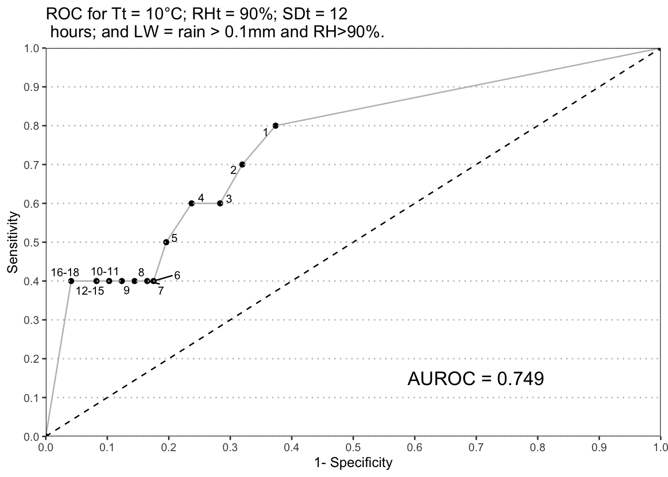
The code
#Save ROC plotting function
save(PlotROC,file = here::here("data", "op_2007_16", "PlotROC.RData"))
Prepare the data for further analysis and check the resulting data frame.
params <- colnames(parameters[, names(parameters) != "model"])
AUROC_data <-
  separate(AUROC_data, model, into =  params, sep = "_")
AUROC_data[, 1:3] <-
  lapply(AUROC_data[, 1:3], as.numeric)
auc_data <- data.frame(AUROC_data)
head(auc_data) %>%
  kable(format = "html") %>%
kableExtra::kable_styling(latex_options = "striped")| rh_thresh | temp_thresh | hours | lw_rh | auc |
|---|---|---|---|---|
| 87 | 10 | 10 | rain | 0.8064433 |
| 87 | 10 | 10 | rainrh | 0.7966495 |
| 87 | 10 | 11 | rain | 0.7680412 |
| 87 | 10 | 11 | rainrh | 0.7997423 |
| 87 | 10 | 12 | rain | 0.7128866 |
| 87 | 10 | 12 | rainrh | 0.7997423 |
auc_datasave(auc_data, file = here::here("data", "op_2007_16", "auc_data.RData"))Packages used.
sessionInfo()## R version 3.6.1 (2019-07-05)
## Platform: x86_64-apple-darwin15.6.0 (64-bit)
## Running under: macOS Mojave 10.14.6
##
## Matrix products: default
## BLAS: /Library/Frameworks/R.framework/Versions/3.6/Resources/lib/libRblas.0.dylib
## LAPACK: /Library/Frameworks/R.framework/Versions/3.6/Resources/lib/libRlapack.dylib
##
## locale:
## [1] en_AU.UTF-8/en_AU.UTF-8/en_AU.UTF-8/C/en_AU.UTF-8/en_AU.UTF-8
##
## attached base packages:
## [1] tools parallel stats graphics grDevices utils datasets
## [8] methods base
##
## other attached packages:
## [1] gt_0.1.0 kableExtra_1.1.0 pander_0.6.3
## [4] here_0.1 mgsub_1.7.1 rcompanion_2.3.0
## [7] R.utils_2.9.0 R.oo_1.22.0 R.methodsS3_1.7.1
## [10] pbapply_1.4-1 remotes_2.1.0 pracma_2.2.5
## [13] ggrepel_0.8.1 readxl_1.3.1 forcats_0.4.0
## [16] stringr_1.4.0 dplyr_0.8.3 purrr_0.3.2
## [19] readr_1.3.1 tidyr_0.8.3 tibble_2.1.3
## [22] ggplot2_3.2.1 tidyverse_1.2.1
##
## loaded via a namespace (and not attached):
## [1] nlme_3.1-140 matrixStats_0.54.0 lubridate_1.7.4
## [4] webshot_0.5.1 httr_1.4.1 rprojroot_1.3-2
## [7] backports_1.1.4 R6_2.4.0 nortest_1.0-4
## [10] lazyeval_0.2.2 colorspace_1.4-1 withr_2.1.2
## [13] tidyselect_0.2.5 compiler_3.6.1 cli_1.1.0
## [16] rvest_0.3.4 expm_0.999-4 xml2_1.2.2
## [19] sandwich_2.5-1 checkmate_1.9.4 scales_1.0.0
## [22] lmtest_0.9-37 mvtnorm_1.0-11 multcompView_0.1-7
## [25] digest_0.6.20 foreign_0.8-71 rmarkdown_1.14
## [28] pkgconfig_2.0.2 htmltools_0.3.6 manipulate_1.0.1
## [31] highr_0.8 rlang_0.4.0 rstudioapi_0.10
## [34] generics_0.0.2 zoo_1.8-6 jsonlite_1.6
## [37] magrittr_1.5 modeltools_0.2-22 Matrix_1.2-17
## [40] Rcpp_1.0.2 DescTools_0.99.28 munsell_0.5.0
## [43] stringi_1.4.3 multcomp_1.4-10 yaml_2.2.0
## [46] MASS_7.3-51.4 plyr_1.8.4 grid_3.6.1
## [49] crayon_1.3.4 lattice_0.20-38 haven_2.1.1
## [52] splines_3.6.1 hms_0.5.0 zeallot_0.1.0
## [55] knitr_1.24 pillar_1.4.2 EMT_1.1
## [58] boot_1.3-22 codetools_0.2-16 stats4_3.6.1
## [61] glue_1.3.1 evaluate_0.14 data.table_1.12.2
## [64] modelr_0.1.5 vctrs_0.2.0 cellranger_1.1.0
## [67] gtable_0.3.0 assertthat_0.2.1 xfun_0.8
## [70] coin_1.3-1 libcoin_1.0-5 broom_0.5.2
## [73] viridisLite_0.3.0 survival_2.44-1.1 TH.data_1.0-10